Week 8 Large Language Models
This tutorial provides a hands-on way to see how large-language-model (LLM) APIs can be integrated into an R research workflow for computational social science. Using the 2018 General Social Survey, we first review tidy data handling, then prompt Mistral AI to act as “synthetic respondents” whose age, sex, race, income, and education match each sampled case.
By contrasting the model’s predicted 2012 presidential vote with the survey’s actual vote distribution and visualising the differences, students learn three key lessons: (1) how to call and parameterize an LLM from R with the {tidychatmodels} grammar; (2) how prompt wording and sampling settings affect generated outputs; and (3) why synthetic text should be interpreted cautiously when compared to real human behavior.
8.1 tidychatmodels Package
In this tutorial, we will use the R package “tidychatmodels”, a recently developed R package by Albert Rapp for LLM API calls, to explore how to integrate LLMs into computational social science research. I also recommend you to read the online documentation for tidychatmodels: https://albert-rapp.de/posts/20_tidychatmodels/20_tidychatmodels
library(devtools)
devtools::install_github("AlbertRapp/tidychatmodels")
library(tidychatmodels)
We also need to following packages for today’s tutorial
library(haven)
library(tidyverse)
library(glue)
library(scales)
library(pins)8.3 LLM as “Synthetic Respondents” for Social Survey: Query
We can now query the LLM! Let’s generate 500 responses from LLM. Let’s first sample 500 real age, sex, race, realinc, and educ combinations from the 2018 GSS data to generate the prompt.
set.seed(42)
n_demo  <- 500
sim_in  <- gss2018 %>% slice_sample(n = n_demo) %>%
           mutate(prompt = pmap_chr(list(age, sex, race,
                                         realinc, educ), make_prompt))
We can check the output of sim_in, which include the 500 sampled real age, sex, race, realinc, and educ combinations and the associated prompt for LLM to respond.
head(sim_in)# A tibble: 6 × 7
age sex race realinc educ pres12 prompt
<dbl> <chr> <chr> <dbl> <dbl> <chr> <chr>
1 46 Male White 72640 16 Obama Imagine you are a 46-ye…
2 66 Male White 30645 20 Obama Imagine you are a 66-ye…
3 65 Male White 8512. 8 Obama Imagine you are a 65-ye…
4 61 Female White 54480 20 Obama Imagine you are a 61-ye…
5 33 Male White 227 12 Obama Imagine you are a 33-ye…
6 28 Male White 24970 18 Obama Imagine you are a 28-ye…Now let’s query the LLM using the customized ask function and store the answer.
library(purrr)
library(pins)
library(stringr)

# ---- helper that returns ONE cleaned token
## out <- … – sends the prompt to the model and gets back the full chat history as a character vector.
## out[length(out)] – keeps only the last element (the assistant’s reply).
-----------------------------
ask_raw <- function(chat, prompt) {
  log_vec <- chat %>%
    add_message(prompt) %>%
    perform_chat() %>%
    extract_chat()              # character vector, one element per turn

  # 1. pick the assistant line (the one that begins with 'Assistant:')
  assistant_line <- log_vec[str_detect(log_vec, "^Assistant:")]

  # if for some reason that pattern isn't found, fall back to the last turn
  if (length(assistant_line) == 0) assistant_line <- tail(log_vec, 1)

  # 2. remove the 'Assistant:' tag, trim white-space
  clean <- str_trim(str_remove(assistant_line, "^Assistant:\\s*"))

  # 3. collapse to length-1 string (in case of accidental line breaks)
  paste(clean, collapse = " ")
}
# ---- wrap it with a 1-request-per-sec rate limiter
## safely() → converts run-time errors (e.g., HTTP 429) into an NA result instead of stopping the loop.
## slowly() → enforces one call per second (rate_delay(1)), satisfying Mistral’s free-tier quota.
## ask_thrott is the error-tolerant, rate-limited wrapper we’ll call inside the loop.
---------------------
ask_safe <- safely(ask_raw, otherwise = NA_character_)
ask_thrott <- slowly(ask_safe, rate = rate_delay(1)) # 1 request / second# ---- prepare pin board and existing progress
## Creates a temporary pins “board”. Everything we cache will live here under the name mistral_sim.
--------------------------
board <- board_temp() # temp folder inside this R session
pin_name <- "mistral_raw"
if (pin_exists(board, pin_name)) {
sim_out <- pin_read(board, pin_name) # resume
done_ids <- sim_out$row_id
} else {
sim_out <- tibble() # start fresh
done_ids <- integer(0)
}# ---- iterate row-by-row with progress bar
## Adds a row_id column so we can track per-row completion, then builds a progress bar for user feedback.
-----------------------------
sim_in2 <- sim_in %>% mutate(row_id = row_number()) # keep row id
todo <- sim_in2 %>% filter(!row_id %in% done_ids) # rows still to query
pb <- progress::progress_bar$new(
format = " querying [:bar] :percent eta: :eta",
total = nrow(todo)
)# Loop body: queries the LLM at a safe rate, appends the new vote (or NA on error) to sim_out, and advances the progress bar.
-----------------------------
for (i in seq_len(nrow(todo))) {
row <- todo[i, ]
ans <- ask_thrott(mistral_chat, row$prompt) # throttled API call
raw <- ans$result # NA if error
sim_out <- bind_rows(sim_out,
row %>% mutate(llm_raw = raw))
pb$tick()
# write/update pin every 25 rows (or on final row)
if (i %% 25 == 0 || i == nrow(todo)) {
pin_write(board, sim_out, pin_name, type = "rds")
}
}Let’s see what we got for the llm responses:
head(sim_out$llm_raw)
[1] "assistant Romney"       "assistant Romney"       "assistant Did_not_vote"
[4] "assistant Did_not_vote" "assistant Did_not_vote" "assistant Did_not_vote"
Apparently, we need to further clean up the raw responses:
sim_out <- sim_out %>%
  mutate(
    # 1. strip the role tag and whitespace
    llm_vote = str_remove(llm_raw, "^assistant\\s*") |> str_trim(),

    # 2. standardise to four canonical values (anything else → NA)
    llm_vote = case_when(
      str_detect(llm_vote, regex("^Obama$",          ignore_case = TRUE)) ~ "Obama",
      str_detect(llm_vote, regex("^Romney$",         ignore_case = TRUE)) ~ "Romney",
      str_detect(llm_vote, regex("^Other$",          ignore_case = TRUE)) ~ "Other",
      str_detect(llm_vote, regex("^Did[_ ]?not[_ ]?vote$", ignore_case = TRUE)) ~ "Did not vote",
      TRUE ~ NA_character_
    )
  )
Let’s compare the actual response distribution with the sythetic ones!
real <- sim_out %>% count(pres12, name = "real_n") %>%
mutate(real_pct = real_n / sum(real_n))
# ── 1. Compute synthetic distribution in numeric form ────────────────
synthetic <- sim_out %>%
filter(!is.na(llm_vote)) %>% # drop invalid / NA answers
count(pres12 = llm_vote, name = "llm_n") %>% # same column name as real
mutate(llm_pct = llm_n / sum(llm_n))
# ── 2. Join & reshape for plotting ───────────────────────────────────
plot_df <- full_join(real, synthetic, by = "pres12") %>% # combine
pivot_longer(cols = c(real_pct, llm_pct), # wide → long
names_to = "source",
values_to = "pct") %>%
mutate(source = recode(source,
real_pct = "Actual GSS",
llm_pct = "LLM (Mistral)"))
# ── 3. Side-by-side bar chart ────────────────────────────────────────
ggplot(plot_df, aes(x = pres12, y = pct, fill = source)) +
geom_col(position = "dodge") +
scale_y_continuous(labels = percent_format(accuracy = 1)) +
scale_fill_manual(values = c("Actual GSS" = "steelblue",
"LLM (Mistral)" = "darkorange")) +
labs(title = "2012 Presidential Vote: Actual vs. Synthetic Respondents",
x = NULL, y = "Share of respondents",
fill = NULL) +
theme_minimal(base_size = 13)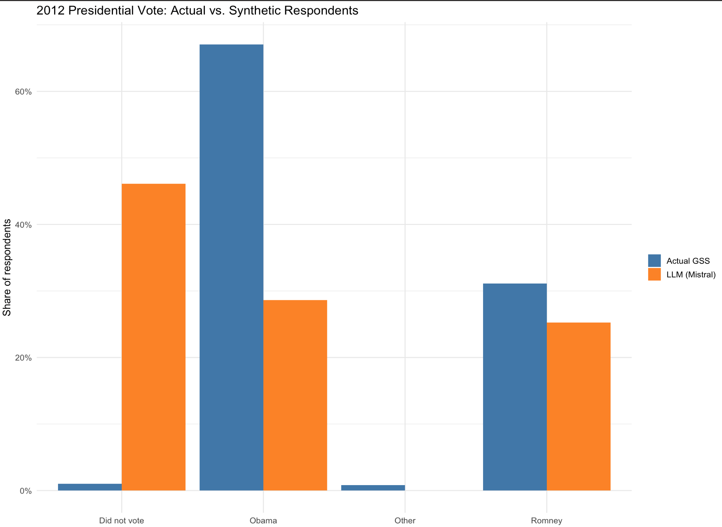 We can compare the alignment using different LLMs.